周志华《机器学习》习题解答：Ch4.3 - 编程实现ID3算法

Python编程实现ID3算法，基于西瓜数据集生成决策树并评估了其好坏。

相关源码托管于Github：PnYuan/Machine-Learning_ZhouZhihua，欢迎访问。

问题回顾

这里采用了自己编程实现和调用sklearn库函数两种不同的方式，详细解答和编码过程如下：（查看完整代码）：

解答内容

数据预分析

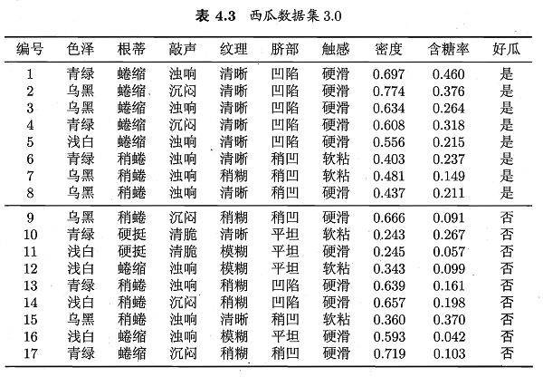
这里由数据表生成.csv文件（注意中文字符的编码格式）。采用pandas.read_csv()读取数据，然后采用seaborn可视化部分数据来进行初步判断。

观察数据可知，变量包含’色泽’等8个属性，其中6个标称属性，2个连续属性。类标签为西瓜是否好瓜（两类）：

下面是一些数据可视化图像：

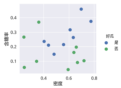
下图是含糖率和密度两个连续变量的可视化图，这个图在之前的练习中也有出现：

下图则是更多的变量两两组合可视化图：

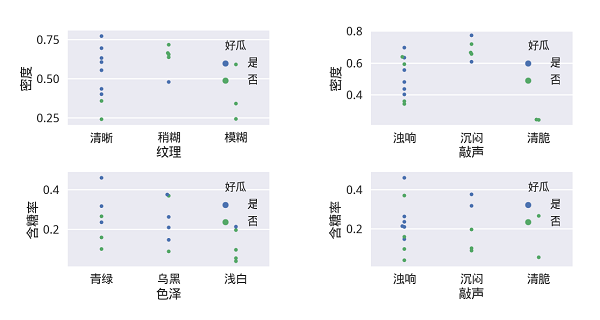
基于可视化手段进行一些分析，看以大概了解数据的分布及其与类别的关系。

编程实现ID3算法

在进行编程之前，先做一些分析如下：

对于树形结构，可以创建节点类来进行操作，根据书p74决策树基本算法，广泛采用递归操作；
对于连续属性（密度、含糖率），参考书p83，对其进行离散化（可采用二分法）；
对于标称属性（色泽、纹理等），考虑Python字典，方便操作其特征类别（如：’色泽’ -> ‘青绿’，’乌黑’，’浅白’）；
由于数据集完整，这里暂不考虑缺值问题（若需考虑，可参考书p86-87的加权思路 -> C4.5算法）；

下面是实现过程：

建立决策树节点类

该节点类包含当前节点的属性，向下划分的属性取值，节点的类标签（叶节点有效，为通用性而保留所有节点类标签）；

样例代码如下：

'''
definition of decision node class

@variable attr: attribution as parent for a new branching 
@variable attr_down: dict: {key, value}
	        key:   categoric:  categoric attr_value 
	               continuous: '<=div_value' for small part
	                           '>div_value' for big part
	        value: children (Node class)
@variable label： class label (the majority of current sample labels)
''' 
class Node(object): 
    def __init__(self, attr_init=None, attr_down_init={}, label_init=None):  
        self.attr = attr_init  
        self.attr_down = attr_down_init
        self.label = label_init

递归实现决策树生成算法主体

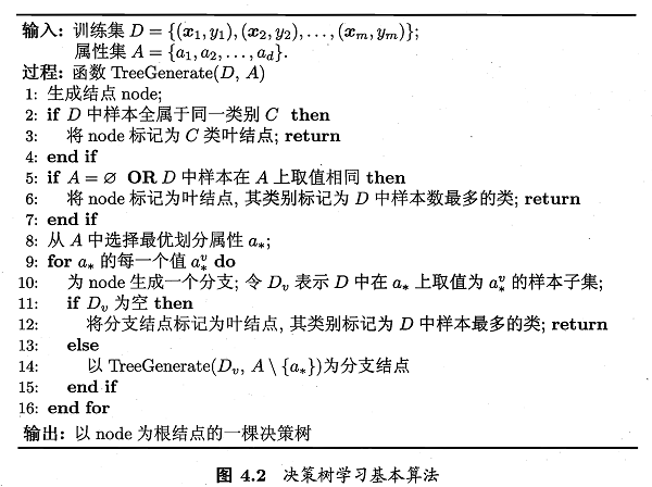
基本的决策树生成算法参照书p74-图4.2，如下所示：

下面是算法主体代码，注意对连续变量和离散变量的不同操作：

def TreeGenerate(df):
	''' 
	Branching for decision tree using recursion 
	 
	@param df: the pandas dataframe of the data_set
	@return root: Node, the root node of decision tree
	'''  
    # generating a new root node
    new_node = Node(None, None, {})
    label_arr = df[df.columns[-1]]
    
    label_count = NodeLabel(label_arr)
    if label_count:  # assert the label_count isn's empty
        new_node.label= max(label_count, key=label_count.get) 
            
        # end if there is only 1 class in current node data
        # end if attribution array is empty
        if len(label_count) == 1 or len(label_arr) == 0:
            return new_node
        
        # get the optimal attribution for a new branching
        new_node.attr, div_value = OptAttr(df)
        
        # recursion
        if div_value == 0:  # categoric variable
            value_count = ValueCount(df[new_node.attr]) 
            for value in value_count:
                df_v = df[ df[new_node.attr].isin([value]) ]  # get sub set
                # delete current attribution
                df_v = df_v.drop(new_node.attr, 1)  
                new_node.attr_down[value] = TreeGenerate(df_v)
                
        else:  # continuous variable # left and right child
            value_l = "<=%.3f" % div_value
            value_r = ">%.3f" % div_value
            df_v_l = df[ df[new_node.attr] <= div_value ]  # get sub set
            df_v_r = df[ df[new_node.attr] > div_value ]
 
            new_node.attr_down[value_l] = TreeGenerate(df_v_l)
            new_node.attr_down[value_r] = TreeGenerate(df_v_r)
        
    return new_node

最优划分属性选择-信息增益判断

ID3算法采用信息增益最大化来实现最优划分属性的选择，这里主要的挑战是离散和连续两种属性变量的分别操作。对于离散变量（categoric variable），参考书p75-77内容实现，对于连续变量（continuous variable），采用书p83-85所介绍的二分法实现。

相关内容如信息熵、信息增益最大化、二分法等可参考书p75-76及p84页内容。

具体的实现代码：查看完整代码。

如下所示为综合了离散类别变量和连续变量的信息增益计算代码实现：

'''
calculating the information gain of an attribution
 
@param df:      dataframe, the pandas dataframe of the data_set
@param attr_id: the target attribution in df
@return info_gain: the information gain of current attribution
@return div_value: for discrete variable, value = 0
               for continuous variable, value = t (the division value)
'''  
def InfoGain(df, index):
    info_gain = InfoEnt(df.values[:,-1])  # info_gain for the whole label
    div_value = 0  # div_value for continuous attribute
    
    n = len(df[index])  # the number of sample

    # 1.for continuous variable using method of bisection
    if df[index].dtype == (float, int):
        sub_info_ent = {}  # store the div_value (div) and it's subset entropy
        
        df = df.sort([index], ascending=1)  # sorting via column
        df = df.reset_index(drop=True)
        
        data_arr = df[index]
        label_arr = df[df.columns[-1]]
        
        for i in range(n-1):
            div = (data_arr[i] + data_arr[i+1]) / 2
            sub_info_ent[div] = ( (i+1) * InfoEnt(label_arr[0:i+1]) / n ) \
                              + ( (n-i-1) * InfoEnt(label_arr[i+1:-1]) / n )
        # our goal is to get the min subset entropy sum and it's divide value
        div_value, sub_info_ent_max = min(sub_info_ent.items(), key=lambda x: x[1])
        info_gain -= sub_info_ent_max
        
    # 2.for discrete variable (categoric variable)
    else:
        data_arr = df[index]
        label_arr = df[df.columns[-1]]
        value_count = ValueCount(data_arr)
            
        for key in value_count:
            key_label_arr = label_arr[data_arr == key]
            info_gain -= value_count[key] * InfoEnt(key_label_arr) / n
    
    return info_gain, div_value

划分训练集和测试集生成模型

首先给出预测函数，采用简单的向下搜索即可实现。查看完整代码。

通过多次划分训练集和测试集，评估出所生成的完全决策树的预测精度，下面是几种不同情况下的结果和分析：

训练集为整个数据样本的情况：
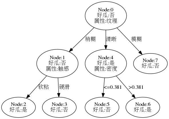
```
accuracy: 1.000  1.000  1.000  1.000  1.000  1.000  1.000  1.000  1.000  1.000  
average accuracy: 1.000
```
此时预测准度为100%，结果证明了题4-1。

采用pydotplus.graphviz绘图库，可以画出这样一棵完全决策树如下图（点击查看绘图程序）：
训练集与测试集各取一半：
```
accuracy: 0.556  0.778  0.333  0.778  0.444  0.333  0.667  0.444  0.778  0.333  
average accuracy: 0.544
```
多次实验预测准度均在55%左右（几乎等同于随机预测），说明此时模型无实用性。
按照K折交叉验证模型（k=5）：
```
accuracy: 1.000  0.000  0.667  1.000  0.000  
average accuracy: 0.533
```
结果精度依然很不理想，可以看到，不同的训练集与测试集的划分导致结果差别很大，这主要是由于数据量太少的缘故。
只分析离散属性：
```
accuracy: 1.000  0.000  0.333  0.667  0.000  
average accuracy: 0.400
```
此时由于特征信息减少，模型更差了。

综上，为提高决策树泛化预测精度，需要进一步对其进行剪枝。

关于剪枝实现可参考下一题。